After completing this module you should be able to:
In Module 2A you learned about commodity futures mainly from an institutional perspective. It is a good idea to reread that module before working through this one to ensure that you have a solid understanding of long and short trading, offsetting and two main roles of a commodity futures (price discovery and risk transfer). In this module we focus on the price discovery role of a commodity futures market. In Module 2G the risk transfer role of commodity futures will be emphasized. After completing this module, which is mainly descriptive, we will return to modeling price dynamics in Modules 2D through 2G, all of which have a strong emphasis on commodity futures and the economic relationship between futures prices and spot prices.
The analysis starts with an examination of the USDA reports, which are used extensively by those who trade futures for agricultural commodities. These reports are kept top secret until the time of their release to minimize the chance of insider trading. One can easily imagine the economic advantage when trading futures from having early access to USDA projections for world supply and demand for the major crops. After discussing the USDA reports we will turn our attention to the economic relationship between the level of overall stocks of a commodity in the market and the price of that commodity. Not surprisingly, price is not very responsive to a change in the level of stocks when stocks are plentiful. When stocks fall below a threshold then the price becomes relatively volatile. The stocks to use ratio is widely used as measure of stock availability. A graph which shows how a commodity's price is positively correlated with the stocks to use ratio emphasizes the important role that stocks play in the analysis of commodity futures.
Following the discussion of stocks, our attention turns to how changes in the composition of global demand and on-going financialization of agricultural commodities are affecting commodity prices. Growth in demand for commodities over the coming years will affect the long term outlook for agricultural commodity prices. The timeframe is too long to be of use for the short-term trading of futures but it is nevertheless important to understand longer term trends in commodity pricing. Livestock consume large amounts of the global grain stock and as such the growth in demand for meat in countries such as China is an important determinant of agricultural commodity price trends. A simple analysis with the Lorenz curve allow us to make some back-of-the-envelope projections about future Chinese demand for meat.
The module concludes with a discussion about the link between energy prices and the prices of agricultural commodities. The main link is through the ethanol and biodiesel markets. The U.S. Renewable Fuel Standard is briefly reviewed to shed light on the massive amount of U.S. corn which is converted into ethanol each year. The demand for corn and thus the price of corn, is connected to the price of crude oil because ethanol and crude oil have positively correlated pricing paths. The same is true for the price linkage between soybeans and crude oil because of the relatively large utilization of soybeans in biodiesel production.
There are many sources of information which are used when trading futures. News about natural disasters, wars, civil unrest, etc. typically impact the futures prices of agricultural commodities through adjustments in current and future commodity supply and demand. When the World Health Organization confirmed the COVID-19 global pandemic in March of 2020, the futures prices of all the major agricultural commodities dropped sharply in tandem with the prices of non-agricultural commodities and equities. The price of wheat made a sharp rebound after it became apparent that consumers were hoarding food and products such as flour was in short supply. News about U.S. government fiscal policy (e.g., scope of quantitative easing) also impacts the price of agricultural commodities because fiscal policy affects economic growth and economic growth is linked to the demand for food, especially meat in developing countries.
One particularly important source of news is in the form of United States Department of Agriculture (USDA) production and demand forecasts. The release of these forecasts typically have an immediate price impact because they affect merchant's storage decisions, which in turn affect both current and future prices of agricultural commodities. A 2019 paper in the Journal of Futures Markets noted that between January of 1991 and May of 2016, price limits were reached and trading for the day was halted 364 times for the case of corn, 692 times for the case of rough rice and 1,036 ties for the case of feeder cattle. Some limit ups or limit downs occurred immediately after the market opened in response to the release of a USDA report the previous evening.
Early in the growing season the number of acres planted to a particular crop is not accurately known. Over time the planted acres estimate become more precise. Weather has a significant impact on planted acres and crop yields. As the growing season progresses, estimates of harvested acres and yield continually change as a result of changes in rainfall, temperature, frost, etc. During the growing season the United States Department of Agriculture (USDA) provides monthly crop production reports. The reports are kept highly confidential and are released at a predetermined time to commodity market traders. If the forecasted production is significantly higher or lower than what traders were expecting then the futures price will adjust rapidly. In some cases the price increase or decrease will reach a daily price change limit and trading will be halted until the next day.
The USDA released a crop production report on August 12, 2021. A summary of the report is provided by (AgWeb). This particular report surprised the market by indicating that corn yields are estimated to be 5 bushels per acre lower than what was previously forecasted. This news caused the price of corn to surge by about 20 cents per bushel. The USDA has become increasingly reliant on satellite data and farmer surveys to construct their yield forecasts. The crop production reports are released monthly during the growing season. The release of USDA reports which contain significant new information typically result in a surge in the volume of trading. In the case of the August 12th announcement, December 2021 corn futures had a volume of 211,985 on the day of the report and 414,290 on the day after the report.
Equally important are the monthly USDA World Agricultural Supply and Demand Estimate (WASDE) reports. For 2021, these reports are released to traders on Jan. 12, Feb. 9, Mar. 9, Apr. 9, May. 12, Jun. 10, Jul. 12, Aug. 12, Sep. 10, Oct. 12, Nov. 9, and Dec. 9. Notice that the August 12th WASDE report was released on the same day (and at the same time) as the USDA crop production report. These means that the news in the crop production report might be offset by the news in the WASDE report and vice versa. For example, weaker than expected export demand combined with lower than expected crop yield may result in only a small price impact even though each one of these reports if released individually would have a sizeable impact.
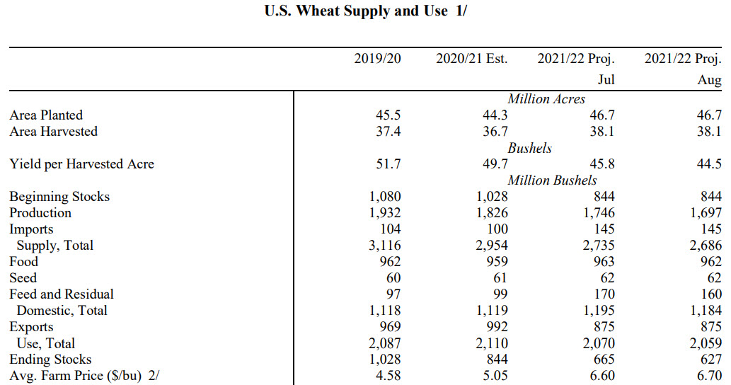
WASDE reports provide forecasts for total U.S. supply and total U.S. demand for each crop as of the end of the crop year (crop years run from September through to the following August). The table below shows the WASDE summary as of August 21, 2021. The first column shows the finalized values for the old crop year (i.e., 2019/2020). The middle column shows the estimates for the current crop year (i.e., 2020/21) and the right column shows the projected values for the next crop year, which begins in September of 2021. The second row (area harvested) multiplied by the third row (yield per harvested acre) gives production, which appears in the fifth column. Production is added to beginning stocks and imports to give total U.S. supply (see the middle of the table). The sum of the next three rows (food, seed and feed) gives total domestic demand. Add exports to domestic demand to get total use (third row from the bottom). Subtract total use from total supply to get ending stocks.
A particularly important forecast in the WASDE report is exports. An unexpected high or low forecast of exports will result in a sizeable price adjustment. For example, in the June 2021 WASDE wheat exports are forecasted to equal 900 million bushels and in the July WASDE report the forecast was lowered to 875 million bushels. The July WASDE report was released on July 12, 2021. Using the historic prices for CME SRW Wheat in (Bar Chart) we see that on July 12, 2021 wheat prices surged by 23.5 cents per bushel. This is strange because we should have expected a softening of the price given the reduced forecast for wheat exports (the June and July WASDE reports show that the forecast for production decreased from 1,898 million bushels in the June report to 1,746 in the July report). Clearly this large decrease in forecasted production was much more important than the reduced exports. Consequently, wheat prices surged upward.
Traders are also influenced by market commentary. And of course the reverse is also true. The following market commentary for corn was provided by Brugler Marketing & Management on June 12, 2020, which is one day after the release of the June 2020 WASDE report: Corn is trading steady to a penny higher this morning after gaining 2 to 3 ½ cents per bushel on Thursday. USDA old crop stocks were raised only 5 million bushels from May to 2.103 bbu. The trade was looking for a 65.1 mbu bump. However, a production cut tied to North Dakota offset 46 mbu of the 50 mbu cut in expected ethanol corn use. For new crop, production and yields were left UNCH, with the larger revisions expected after the June 30th report. Globally, new crop ending stocks were cut to 337.87 MMT. South American corn production was UNCH. The Export Sales report showed old crop corn sales on the week ending June 4 were 26.01 mbu. New crop sales came in at 1.02 mbu. Accumulated commitments are 15% below a year ago, a 1 ppt improvement wk/wk.
We see the USDA raised their estimate of corn stocks coming into the 2019/2020 crop year by 5 million bushels, which is much less than the 65.1 million bushels that traders were expecting. This unexpected announcement would put upward pressure on the price. Traders were expecting demand for corn in ethanol production to decrease by 50 million bushels but this reduction was largely offset by a 46 million bushel reduction in North Dakota wheat production. There was no change in the forecast for new crop production but new crop ending stocks were cut. Overall, the combined effect of these forecast adjustments were minimal because the price of corn only increased by 2 to 3.5 cents per bushel after the release of the report.
For storable commodities it is important to view available supply as incoming stocks plus current production, and outgoing stocks as available supply minus current usage. If current usage outstrips current production then the stockpile will run down. The stock pile is very important because it stabilizes price. In the absence of a sizeable stockpile, a drought or an unanticipated surge in demand would send prices soaring. The fact that the supply shortfall or the demand surge can be addressed by drawing down the stock pile stabilizes the price over time. As the stock pile depletes the risk of future shortages increases and the price increases accordingly. The market does not keep an excessively large stock pile because doing so is costly both in terms of spoilage and the physical cost of warehousing the commodity.
Recognizing the important role of stocks, various governments maintain public stockpiles of food commodities. If they are set up and managed properly, a government stockpile can be effective at maintaining price stability and ensuring food security. Unfortunately, public stockpiling schemes often fail because governments cannot resist using them as sources of farm income support. The government scheme typically involves buying commodity and placing it a public stockpile when the market price falls below a lower threshold, and releasing public stocks back into the market when the price rises above an upper threshold. The lower threshold is often set too high and the public stockpile increases excessively. When governments try to deplete the stockpile they end up depressing the market price. You can read more about public stockpile and the associated controversies here.
The graph below shows monthly WASDE forecasts of ending corn stocks and the average farm price for the crop year. Notice the rapid price increase over the years 2011 - 2013 in response to depleting stocks. Conversely, corn stocks rose quite rapidly and the average farm price of corn fall sharply during the 2014 - 2017 period. Corn stocks and price were both relatively stable between 2017 and early 2020. Beginning in late 2020, and throughout the first half of 2021, corn stocks rapidly depleted and prices simultaneously rose. The increase in the market price of corn during the first six months of 2021 was much stronger than that shown in the graph, which is a measure of yearly average price. In general the graph makes it clear that the size of the corn stockpile is and important determinant of both the price level and the level of price volatility.

The stocks to use ratio is a measure of the level of stocks relative to annual use of the commodity. The figure below shows that for the corn and wheat this ratio has followed a flat trend line since the 1960s. The long term average stocks to use ratio is about 25 percent for corn and about 30 percent for wheat. According to the FAO, a major cause for the very large spike in food prices in 2007 - 2008 was unusually low stock to use ratios for the major grains. For example, "The ratio of world cereal ending stocks in 2007/08 to the trend world cereal utilization in the following season is forecast to fall to 18.8 percent, the lowest in 3 decades." As well, "The ratio for wheat is forecast to fall to 22.9 percent, well under the 34 percent level observed during the first half of the decade."
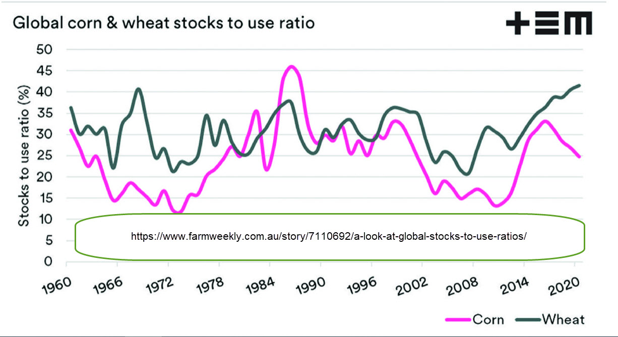
The reason for the rapid fall in the stocks to use ratios in 2006 - 2008 was a combination of low production due to drought in key regions, and strong demand, particularly in large population countries such as China and India. You should spend some time reading about the 2007 - 2008 world food price crisis in Wikipedia.
The figure below shows the average monthly price of a nearby corn futures contract and the average monthly S&P 500 stock price index. The price of corn is clearly much more volatile than the stock price index. There is some evidence that the two series respond to the same shock but in general the correlation is weak. According to a 2019 blog, corn and wheat have a correlation with the S&P 500 of about 0.2. The low correlation of agricultural futures with major stock market indexes have resulted in the rapid growth of agricultural exchange trade funds (ETFs). The term "financialization" of agricultural commodities refers to the large scale investment in agricultural ETFs by hedge funds and retail investors over the past 15 years. Critics argue that this financialization has the potential to drive food prices higher and make them more volatile. There have been many studies which empirically investigated this claim and to date supporting evidence has been weak. We will examine these ETFs in greater detail in a later module.
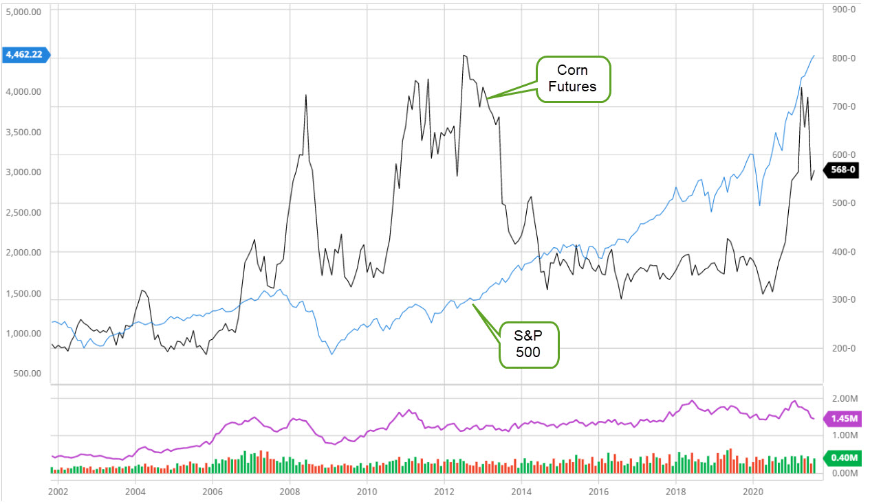
The above figure shows the dramatic increase in corn prices in 2007 - 2008, and then again in 2011 - 2013. Common explanations for these price surges include: production shortfalls, export embargoes, the increasing use of corn and soybeans for biofuels, the financialization of agricultural commodities and a surge in demand for agricultural commodities by China and other rapidly-growing economies. The last reason is explained by noting that as per-capita income increases in China and other countries, households will demand more meat which in turn implies higher demand for feed grains. Subsequent studies have shown that the surge in demand explanation is generally not true.
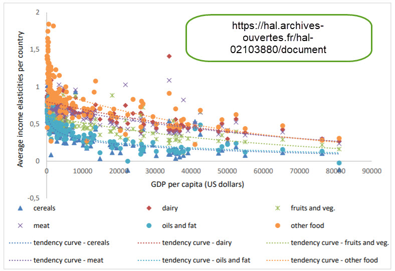
Even though the demand surge argument is generally not true for the 2007-2008 spike in food prices it is nevertheless still useful to examine the outlook for longer term growth in food demand. The diagram below shows that countries with a higher GDP per capita generally have lower food income elasticities. For example, in a poor country with per capita GDP of US$5000 per year the income elasticity for meat is about 1 whereas in a wealthy country with a per capital GDP of US$55,000 per year the income elasticity of meat is about 0.5. This outcome is consistent with Engel's Law, which states that the share of expenditures on food declines with higher income. If global income inequality continues to increase then according to Engel's Law the increase in demand for food will primarily be driven by an increase in the global population. On the other hand, if there is convergence in economic growth across countries, and in recent years this seems to be the case, then we should expect an moderately strong increase in per capita demand for food as well as an increase in demand due to an increase in the global population. In this second case the per capita demand will be biased away from starch foods and towards more meat and protein, which has obvious implications for the long term prices for livestock and feed grains.
Meat Demand Case Study
In this section a simple model of growth in the demand for meat in China is used to illustrate how the distribution of income growth across households is a key determinant of the overall growth in meat demand. The model assumes a fixed population and thus focuses on increases in the consumption of meat per household. This example is highly stylized and the parameter values should be viewed as very rough estimates of the true parameter values. Nevertheless, the results effectively show why income inequality is an important determinant of future growth in Chinese meat demand.
Recent statistics reveal that average per capita meat consumption in China is about 56 kg per year. Assuming that the price of meat across all categories averages to US$10 per kg it follows that average meat expenditures per capita are approximately US$500 per year. The average per capita income in China is about US$8,800, and we will assume that 30 percent of this income is spent on food. This means that meat expenditures relative to total food expenditures is about 500/(0.3*8800) = 0.19 or 19 percent. This ratio is similar to the U.S. ratio where the typical household spends about $900 per year on meat products and about $4600 per year on overall groceries.
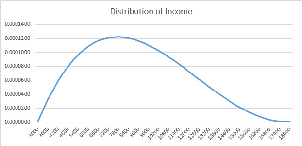
We expect the distribution of income across Chinese households to have a long right tail. To keep things simple, assume for the base case that income varies from a low of US$3000 to a high of US$18,000, and between these two extreme values per capita income follows a beta distribution, as shown in the figure below. The standard deviation of income for this base case scenario is 2940. The standard deviation relative to the mean is 2940/8800 = 0.334 or about 33 percent.
In the economic development literature the Lorenz curve is generally used to graphically illustrate income inequality across households. The figure below shows the Lorenz curve for the base case (i.e., previous diagram). The diagonal line represents a situation where all households have equal income. The extent that the Lorenz curve lies below the diagonal line is a measure of income inequality. The Lorenz curve is summarized by the Gini Coefficient, which is given by area A divided by area A + area B. The Gini coefficient ranges from 0 for the case of perfect income equality to 1 for the case where one person in the country has all of the wealth. In this base case the Gini Coefficient is about 15 percent, which is well below the 0.465 estimate of the real-world Chinese Gini Coefficient. The lack of a long right tail in the current model is the reason for this large discrepancy.

Assume that the quantity of meat consumed, M, is given by M = a + bln(E) where E is household expenditures on all food and ln() is the natural logarith function. Using this equation, the meat expenditure elasticity, (dM/dE)(E/M), can be expressed as η = b/M. Invert this equation to get b = ηM, and now rewrite the equation as a/M = 1- ηln(E). The table below shows the mean value of M (annual quantity of meat consumed) is 56, and mean annual food expenditures, E, are 2640. Substituting in these values into the previous equation gives us a = -275 and b = 42.
We previously assumed that 30 percent of household income is devoted to food expenditures, which implies E = 0.3*I. Our equation can therefore be written as M = -275 + 42ln(0.3I). Let EM denote meat expenditures. Assuming the price of meat is $9/kg, the previous equation can be rewritten as EM = -2475 + 378ln(0.3) + 378ln(I). This equation reduces to:
EM = -2930 + 378ln(I)
| Parameter | Value |
|---|---|
| Mean M (kg) | 56 |
| Mean E ($) | 2640 |
| Mean I ($) | 8,800 |
| Price ($/kg) | 9 |
| η | 0.75 |
If we divide the previous equation through by I we get an expression which shows the share of per capita income which is spent on meat:
EM/I = [-2930 + 378*ln(I)]/I.
A graph of this share equation is presented below. Notice that for very poor households, the share of income devoted to meat initially increases as the household receives higher income. However, quite soon Engel's Law prevails and the share of per capita income which is devoted to meat decreases with higher income. The shape of this schedule is very important because it determines how overall meat demand for the country will increase as the country becomes wealthier. This is explained in greater detail below.

We can now use the model to examine increases in meat demand under two alternative income growth scenarios. The first scenario is called pro-poor and the second scenario is called pro-rich. In both cases mean per capital income for China increase from US$8,800 to US$9,500. In the pro-poor scenario this increase results from minimum income raising from US$3,000 per capita to US$6,000 per capita, and maximum income remains fixed at US$18,000. In the pro-rich scenario this increase results from maximum income raising from US$18,000 to US$25,000, and minimum income remains fixed at US$3,000 per capital. Starting from a base case value of 2940, the standard deviation of income decreases to 1946 in the pro-poor scenario and rises to 3601 in the pro-rich scenario.
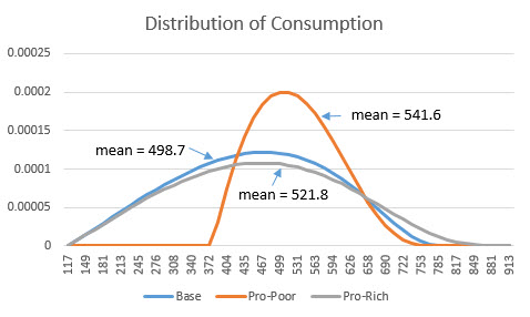
The Figure below shows the distribution of consumption for the base case and the two income growth scenarios. The obvious result is that the pro-poor scenario has resulted in a strong shift of the distribution of consumption to the right. In contrast, the pro-rich scenario has resulted in a very weak shift of the distribution of consumption to the right. Starting with base case expenditures on meat equal to US$498.7 per year, mean meat expenditures increases to US$ 541.6 per capita with the pro-poor scenario and US$521.8 with the pro-rich scenario. This difference may not seem particularly large but when aggregated over 1 billion consumers, the difference in overall meat demand for the two scenarios is highly noteworthy.
The differential impact on meat demand across the two scenarios can be fully attributed to the downward sloping meat expenditure share equation. For each extra dollar earned by a poor person, a sizeable fraction of that dollar is spent on meat. In contrast, for higher income person a relatively small fraction of the marginal dollar of income is spent on meat. Thus, the pro-poor scenario which primarly raises low incomes has a much larger effect on meat demand as compare to the pro-rich scenario, which primarily raises high incomes.
Agricultural commodities are widely used in the production of biofuels, primarily ethanol and biodiesel. This utilization is widely believed to create a link between the price of energy and the price of agricultural commodities. The concern is that the shifting of agricultural commodities into biofuel production has increased the price of food and has made food prices more volatile. Of particular interest is the role that biofuels played in the 2007-2008 food price crisis, and its potential contribution to future food price crisis. In this section we will review some summary statistics of biofuel production and perform some simple time series analysis in an attempt to identify a causal effect of the price of diesel on the price of soybean oil.
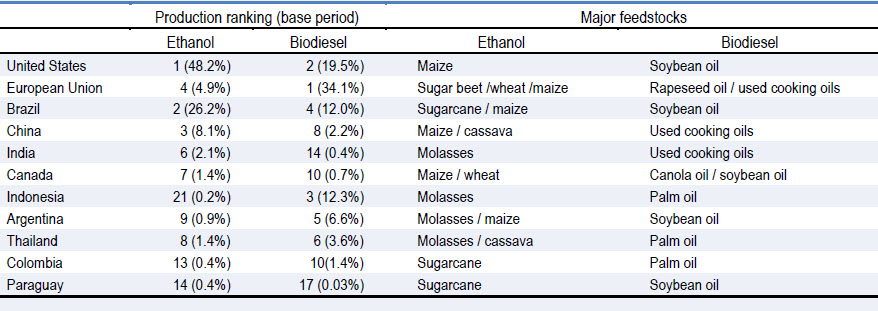
The table below provides a ranking of countries according to their production of biofuels. The U.S. is the number 1 producer of ethanol, and within the U.S. maize/corn is the primary feedstock. The EU is the number 1 producer of biodiesel and rapeseed oil is the primary feedstock. Brazil and China are the number 2 and number 3 producers of ethanol, with sugarcane, maize and cassava serving the primary feedstock. The U.S. and Indonesia are the number 2 and number 3 producers of biodiesel with soybean oil and palm oil, respectively, serving as the primary feedstock.
The U.S. Renewable Fuel Standard Program was created in 2015 in an attempt to reduce its reliance on imported oil and to reduce greenhouse gas (GHG) emissions. Fracking technology has largely made the U.S. self sufficient in fossil fuels but a strong farm lobby has preserved the large scale production of ethanol. The GHG benefits of biofuel production have largely not materialized due to the large amount of energy-intensive farm inputs which are required to produce the primary inputs of biofuels (i.e., corn and soybeans).
In 2020 the U.S. produced 13.675 billion gallons of ethanol and 2.459 billion gallons of biodiesel. This large-scale production of ethanol was produced from about 5.4 billion bushels of corn. In 2020 about one third of the U.S. corn crop was allocated to the production of ethanol. About 85 percent of the 2.459 billion gallons of biodiesel are produced from 1.4 billion bushels of soybeans. In 2020 about 32 percent of U.S. soybean production was allocated to the production of biodiesel.
The U.S. Renewable Fuel Standard Program dictates the total amount of renewable fuel which must be used in the U.S. each year. The maximum fraction of ethanol in gasoline is 10 percent for older cars and 15 percent for new cars. Overall, about 10 percent of the gasoline consumed in the U.S. consists of ethanol. Diesel burning cars and trucks have a higher tolerance for biofuel blending. The most common diesel fuel is B-20, which typically contains between 6 and 20 percent biodiesel.
The legislated use of biofuels means that the prices of biofuels can evolve over time quite differently than the price of gasoline or diesel. The table below shows that biofuels command a sizeable premium over their fossil fuel counterparts. As well, the table clearly shows that even on a month-to-month basis the percent difference between the price of regular fuels and their biofuels counterparts can vary widely (note that the price of ethanol is reported on an energy adjusted basis). These results are important because they show there is less reason to believe there will exist a direct link between the price of energy and the price of agricultural commodities such as corn and soybeans.
| Month | Gasoline | Ethanol | % Difference | Diesel | Biodiesel | % Difference |
|---|---|---|---|---|---|---|
| Jan, 2021 | $1.63 | $2.31 | 41.7% | $3.15 | $3.85 | 22.2% |
| Feb, 2021 | $1.92 | $2.58 | 34.4% | $2.75 | $4.92 | 78.9% |
| Mar, 2021 | $2.20 | $2.79 | 26.8% | $3.15 | $5.00 | 58.7% |
| Apr, 2021 | $2.15 | $3.21 | 49.3% | $3.13 | $4.32 | 38.0% |
| May, 2021 | $2.24 | $3.91 | 74.6% | $3.22 | NA | NA |
| Jun, 2021 | $2.53 | 3.78 | 49.4% | $3.29 | $5.99 | 82.1% |
Time Series Analysis
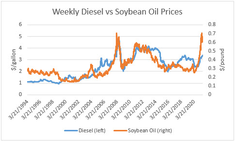
The graph below shows the average weekly futures price of soybean oil and the average weekly retail price of diesel fuel from March of 1994 to August of 2021. Of interest is the extent that changes in the price of diesel fuel cause changes in the price of soybean oil. Eyeballing the data shows a moderately strong correlation. Our goal in this section is to use some elementary time series analysis to be more precise in our characterization of the pricing relationship.
As a starting point we can regress the price of soybean oil (measured in dollars per pound) on the price of diesel fuel (measured in dollars per gallon) and then check if the regression coefficient is statistically significant. The regression was performed in Excel using the Data - Data Analysis - Regression tool. A screen capture of the results are presented below. We see a moderately high value of the R2 value and a highly statistically significant coefficient estimate -- the p value is very close to zero. So far so good in establishing that the price of diesel fuel has an impact on the price of soybean oil.
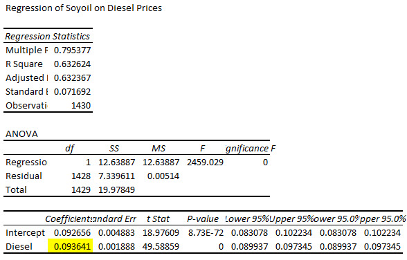
How should we interpret the coefficient estimate of 0.0936? In the 2020/2021 FRE 501 class the price of 100 percent biodiesel measured in dollars per gallon was regressed on the price of regular diesel fuel measured in dollars per gallon, and the following regression equation was obtained: PBD = 1.572 + 0.657PD. If this equation is divided by 7.6 because there are 7.6 pounds per gallon for either regular diesel or biodiesel, then the regression equation can be rewritten as PBD* = 0.207 + 0.086D where PBD* is the price of biodiesel measured in dollars per pound. This equation can be compared directly to the regression presented in this class. The intercept term is a bit different (0.093 versus 0.097) but the slope estimates are very close (0.094 versus 0.086). Again this should give us confidence that we are on the right track with our model.
It time series analysis data series must be stationary when running regression to avoid the risk of estimating spurious (and thus meaningless) deterministic or stochastic trends in the data. One important exception to this rule is that we are allowed to run regressions with non-stationary data provided that both data series are co-integrated. If the two data series are co-integrated then the residuals from the regression are stationary. The diagram below shows a graph of the residuals from the previous regression. Cointegration implies that the data should look like white noise and thus contain no autocorrelation. The graph appears to reveal moderate autocorrelation, and thus it may not be the case that the price of diesel and the price of soybean oil are co-integrated. With such an outcome we cannot trust our previous regression results and therefore can draw no conclusions about whether or not the price of diesel affects the price of soybean oil.
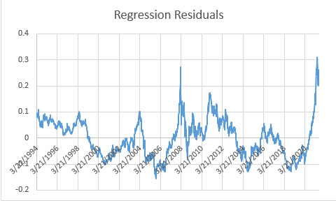
It is beyond the scope of this analysis to describe the specific Augmented Dickey Fuller (ADF) test for determining whether or not the residuals or stationary. In a nut shell, the first difference of the residuals is regressed on the lagged value of the residual and the lagged value of the first difference. The ADF test statistic is the t statistic on the estimated coefficient of the lagged residual. In this particular case the t statistic is -2.750. The null hypothesis is that residuals are non-stationary. The critical values for large samples are -3.43 for a 1 percent test and -2.86 for a 5 percent test. Noting that the absolute value of -2.750 is less than the absolute value of both -3.43 and -2.86 it follows that we are not able to reject the null hypothesis of non-stationary residuals and thus not able to claim that that the two prices are cointegrated. It is likely that rejection is possible at the 10 percent level. Thus, we can conclude that despite the high R2 and highly significant estimate of the regression coefficient, there is only weak evidence that the price of diesel impacts the price of soybean oil.
This module focused on what is known as the fundamental analysis of commodity prices. Economists believe that fundamental analysis is essential for successfully trading commodity futures, whether it be for hedging or for speculation. Others believe that technical analysis (e.g., charting past data) is the best way to play the futures, especially for speculation. The following blog has an interesting discussion about the tradeoffs when using technical versus fundamental analysis for trading. The general conclusion is that those who use a combined approach of fundamental and technical analysis are likely to earn the highest profits from trading futures. Economists who believe in the efficient market hypothesis generally discount the value of technical analysis. This is because the efficient market hypothesis tells us that the current price reflects all available information, and as such past prices have no predictive capabilities.
Planted acreage forecasts and short and long term weather forecasts, especially frost and hail, are particularly important for fundamental analysis. It is relatively easy to identify price surges in orange juice futures in responses to forecasts for a deep freeze in Florida during the orange growing season. Traders have a growing number of opportunities to subscribe to satellite data services, which predict acres planted of the major crops and signs of weak or strong crop yield potential. With climate change creating more volatile weather we will likely see an associated increase in futures price volatility during the crop growing season. And with higher yield variability due to climate change, we are likely to see higher levels of annualized commodity price volatility.
An often overlooked reason for unexpected changes in commodity prices is policy risk and political risk. China's overnight banning of Canadian canola imports in apparent retaliation for Canada's role in the December, 2018 arrest and detention of Meng Wanxhou, created a rapid and very large decrease in the price of Canadian canola. Similarly, in 2014 the U.S. enacted "Country of Origin" (COOL) labeling requirements. This new policy put Canadian livestock producers at a large disadvantage when exporting live animals to the U.S., and Canadian livestock prices fall sharply in response. The rapid ban on Canadian exports of beef in response to 2003 positive test results for bovine spongiform encephalopathy ("mad cow disease") also resulted in a sharp and prolonged price drop for beef producers.